Einstein Relation (Kinetic Theory)

In physics (namely, in kinetic theory) the Einstein relation (also known as Einstein–Smoluchowski relation) is a previously unexpected connection revealed independently by Albert Einstein in 1905 and by Marian Smoluchowski (1906) in their papers on Brownian motion. Two important special cases of the relation are:

$D = {{\mu_q \, k_B T}\over{q}}$ (Diffusion of charged particles)

$D=\frac{k_B T}{6\pi\,\eta\,r}$ ("Einstein-Stokes equation", for diffusion of spherical particles through liquid with low Reynold's number)

Where

D is the diffusion constant,
q is the electrical charge of a particle,
μ_q, the electrical mobility of the charged particle, i.e. the ratio of the particle's terminal drift velocity to an applied electric field,
$k B$ is Boltzmann's constant,
T is the absolute temperature,
η is viscosity
r is the radius of the spherical particle.

The more general form of the equation is: $D = \mu \, k_B T$ Where the "mobility" μ is the ratio of the particle's terminal drift velocity to an applied force, μ = v_d / F. This equation is an early example of a fluctuation-dissipation relation. It is frequently used in the electrodiffusion phenomena. Derivations of Special Cases from General Form Electrical Mobility Equation For a particle with charge q, its electrical mobility μ_q is related to its generalized mobility μ by the equation μ_q=μq. Therefore, the general form of the equation $D = \mu \, k_B T$ is in the case of a charged particle: $D = \frac{\mu_q \, k_B T}{q}$ Einstein-Stokes Equation In the limit of low Reynolds number, the mobility

μ

is the inverse of the drag coefficient

γ

. For spherical particles of radius

r

, Stokes' law gives $\gamma = 6 \pi \, \eta \, r,$ Where

η

is the viscosity f the medium. Thus the Einstein relation becomes

$D=\frac{k_B T}{6\pi\,\eta\,r}$

Semiconductor In a semiconductor with an arbitrary density of states the Einstein relation is $D = {{\mu_q \, p}\over{q {{d \, p}\over{d \eta}}}}$ Where

η

is the chemical potential and p the particle number. Proof of General Case (This is a proof in one dimension, but it is identical to a proof in two or three dimensions: Just replace d/dx with $\nabla$ . Essentially the same proof is found in many places, for example see Kubo.) Suppose some potential energy U creates a force on the particle

F = - d U / d x

(for example, an electric force). We assume that the particle would respond, other things equal, by moving with velocity

v = μ F

. Now assume that there are a large number of such particles, with concentration

f (x)

as a function of position. After some time, equilibrium will be established: The particles will "pile up" around the areas with lowest U, but will still be spread out to some extent because of random diffusion. At this point, there is no net flow of particles: The tendency of particles to get pulled towards lower U (called the "drift current") is equal and opposite the tendency of particles to spread out due to diffusion (called the "diffusion current"). The net flow of particles due to the drift current alone is: $J_{\mathrm{drift}}(x)=\mu \, F(x) \, f(x) = -f(x) \mu \, dU/dx$ i.e. the number of particles flowing past a point is the particle concentration times the average velocity. The net flow of particles due to the diffusion current alone is, by Fick's laws: 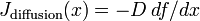$J_{\mathrm{diffusion}}(x)=-D \, df/dx$ (the minus sign means that particles flow from higher concentration to lower). Equilibrium requires:

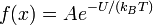$0 = J_{\mathrm{drift}} + J_{\mathrm{diffusion}} = -f(x) \mu \, dU/dx - D \, df/dx$

In equilibrium, we can apply thermodynamics, in particular Boltzmann statistics, to infer that: $f(x) = A e^{-U/(k_B T)}$ Where A is some constant related to the total number of particles. Therefore, by the chain rule, $df/dx = \frac{-dU/dx}{k_B T} f(x).$ Finally, plugging this in: $0 = J_{\mathrm{drift}} + J_{\mathrm{diffusion}} = -f(x) \mu \, dU/dx - D \, df/dx = -f(x)dU/dx \left(\mu-\frac{D}{k_B T}\right)$ Since this equation must hold everywhere, $\mu=\frac{D}{k_B T}.$

Fuente: http://en.wikipedia.org/wiki/Einstein_relation_(kinetic_theory)

Nombre: Rodriguez B. Joiver I. Asignatura: CRF